Bayesian Machine Learning: A Deep but Friendly Introduction

02 February 2025
Tags: Statistics Bayesian Machine Learning Machine Learning Data Science Python

The first time you hear about Bayesian Machine Learning, it might sound a bit intimidating. Maybe you’ve even encountered it in the never-ending “Bayesian vs. Frequentist” debate and decided it was safer to steer clear altogether. But here’s the thing: Bayesian ML isn’t as scary as it’s made out to be. In fact, many of its ideas have familiar counterparts in classical (frequentist) machine learning, and once you see the connections, it all starts to click!

At its core, Bayesian ML is just machine learning with uncertainty baked in. While classical ML methods give you a single “best” set of parameters, Bayesian tell you how confident the model is in those parameters. Instead of point estimates, we get access to full distributions!

In this post, we’ll take a deep but gentle dive into Bayesian Machine Learning. We’ll start with the fundamentals, Bayes’ Theorem, and then build up to Bayesian inference in machine learning. Along the way, we’ll explore:

• Why Bayesian ML is useful and how it helps quantify uncertainty
• How Bayesian ML connects to classical ML (spoiler: they’re more similar than you think!)
  • Are priors a dangerous source of bias?
• How to implement Bayesian Linear Regression and Bayesian Neural Networks in Python

By the end of this post, you should have a good understanding of the basics of Bayesian Machine Learning, as well as some code to get started in your own projects. So, let’s get started!

1. Why Bayesian Machine Learning?

You might be wondering: why bother with Bayesian machine learning at all? After all, classical machine learning methods like linear regression, decision trees, and neural networks already work pretty well. So what’s the deal with Bayesian methods? The answer lies in uncertainty.

In classical machine learning, when we train a model, we often end up with a single set of “best” parameters (like the coefficients in linear regression or the weights in a neural network). But here’s the thing: how confident are we in those parameters? What if there are other parameter settings that could explain the data just as well? Classical methods typically don’t give us a direct way to answer those questions.

Bayesian machine learning, on the other hand, doesn’t just give you one “best guess” for the parameters. Instead, it provides a full distribution over possible parameter values (the posterior). This means we’re not just saying, “Here’s the best model,” but rather, “Here’s the range of plausible models, and here’s how confident we are about each one.”

Being able to provide confidence intervals is a game changer. In many fields, it’s not enough to simply make a prediction: we also need to communicate how confident we are in that prediction (this is called uncertainty quantification). Take finance, for example: knowing not just the most likely outcome but also the range of possible outcomes can make a huge difference in assessing risk.

The benefits go beyond specific use cases. For you, as an ML practitioner, being able to share both predictions and their uncertainties is a massive win when communicating with stakeholders, whether they’re technical or non-technical. By presenting both the “what” and the “how sure,” you’re providing a fuller, more transparent picture. This builds trust, fosters clarity, and makes it far more likely that your insights will lead to real-world impact with actionable steps.

There is actually a method called Conformal Prediction (CP) which has gained a lot of popularity lately! It is a framework for uncertainty quantification that generates statistically valid prediction intervals for any type of point predictor (statistical, machine learning, deep learning, …) under the assumption that the data is exchangeable. I might write about it in the near future!

2. Bayes Theorem

Let’s get our hands dirty with some math and introduce the famous Bayes’ theorem! If you’re already an expert on this, feel free to skip this section (it’s always good to refresh our memory though). The formula itself is quite straightforward to derive. It all starts with the relationship between joint and conditional probabilities:

which reads, the probability of both A and B happening (denoted as \(P(A \cap B)\)) is equal to the probability of B happening (\(P(B)\)), multiplied the probability of A happening knowing that B happens (\(P(A | B)\)).

Now, it’s always easier to make sense of this with a practical example:

• Let \(A\) represents “it is rainy” \(\rightarrow P(A)\) is the probability that it is rainy.
• Let \(B\) represents “it is foggy” \(\rightarrow P(B)\) is the probability that it is foggy.

If we plug these into the formula, the probability of it being rainy and foggy, \(P(A \cap B)\), is simply the probability that it is foggy (\(P(B)\)) multiplied by the probability that is is rainy given that it’s foggy \(P(A | B)\)

Let’s work with numbers to make this more concrete: say it is foggy on 50% of days, and on those foggy days, it is rainy 20% of the time. Then, the probability that it is both foggy and rainy is:

Now, here is the key insight: the probability of it being rainy and foggy is the same as the probability of it being foggy and rainy. In other words, \(P(A \cap B) = P(B \cap A)\). Using this symmetry, we can rewrite:

From here, if we isolate \(P(A \mid B)\) and rearrange terms a bit, we arrive at:

And there you have it: Bayes’ Theorem!

Not too bad, right? Once you break it down step by step, it’s just basic probability relationships coming together. Now that we’ve got this foundation, we can start building on it.

3. Bayes’ Theorem and Machine Learning

Now that we’ve got Bayes’ Theorem under our belt, let’s connect it to machine learning. At its core, machine learning involves two key ingredients:

• The Data: We start with an observed dataset of \(M\) observations, \(\mathcal{D}=\{\mathbf{x}^i; y_i\}\), where each \(\mathbf{x}^i = (x^i_1, x^i_2, ..., x^i_M) \in \mathcal{R}^M\) represents the feature vector for the \(i^{th}\) observation, and \(y_i \in \mathcal{R}\) is the corresponding target value (what we’re trying to predict).
• The Model: We use a model \(\mathcal{M}_{\hat{\boldsymbol{\theta}}}\) to capture the relationship between the features and the target. This model is defined by a parameter vector \(\hat{\boldsymbol{\theta}} = (\hat{\theta}_1, \hat{\theta}_2, ..., \hat{\theta}_N)\in \mathcal{R}^N\). For example, in a linear model, \(\hat{\boldsymbol{\theta}}\) would be the set of linear coefficients we want to learn.

Now, here’s where Bayes’ Theorem comes into play. If we plug the data and model into Bayes’ formula, we get:

(Notice the lowercase “p” here: we’re dealing with continuous distributions.)

Each term in this equation has a specific meaning:

• \(p(\hat{\boldsymbol{\theta}} | \mathcal{D})\) is the posterior, which tells us the probability of parameters \(\hat{\boldsymbol{\theta}}\) after we have seen the data;
• \(p(\mathcal{D} | \hat{\boldsymbol{\theta}})\) is the likelihood, which tells us how well the model explains the data given a specific set of parameters \(\hat{\boldsymbol{\theta}}\).
• \(p(\hat{\boldsymbol{\theta}})\) is the prior, which represents our beliefs about the parameters before seeing the data. For instance, we might believe the parameters are likely to be close to zero (I’ll cover in practice how to handle this later on).
• \(p(\mathcal{D})\) is the evidence, which is essentially a normalizing constant. For most practical purposes, we don’t need to worry too much about this term.

So, what’s the goal in Bayesian machine learning? It’s to find the posterior \(p(\hat{\boldsymbol{\theta}})\). Once we have that, we can use it to make predictions \(\tilde{y}\) on new, unseen data \(\tilde{\mathbf{x}}\).

where \(\mathcal{M}_{\hat{\boldsymbol{\theta}}}(\tilde{\mathbf{x}}) = \tilde{y}_{\hat{\boldsymbol{\theta}}}\) is the predicted value obtained from input features \(\tilde{\mathbf{x}}\) given parametrization \(\hat{\boldsymbol{\theta}}\). Let’s break this down in plain language:

The prediction \(\tilde{y}\) is a weighted average of all possible predictions \(\tilde{y}_{\hat{\boldsymbol{\theta}}}\). The “weights” come from the posterior \(p(\hat{\boldsymbol{\theta}} | \mathcal{D})\), which tells us how likely each set of parameters \(\hat{\boldsymbol{\theta}}\) is, given the observed data.

In practice, computing the integral above directly is often infeasible. The posterior distribution \(p(\hat{\boldsymbol{\theta}} | \mathcal{D})\) is usually too complex to solve analytically, especially when dealing with high-dimensional parameter spaces. So what do we do? We approximate it. Instead of computing the full integral, we sample from the posterior using numerical methods. This leads us to a practical way of estimating predictions:

where \(Q\) is the number of samples and \(\hat{\boldsymbol{\theta}}_1, \hat{\boldsymbol{\theta}}_2, ..., \hat{\boldsymbol{\theta}}_Q\) parameter samples drawn from the posterior \(p(\hat{\boldsymbol{\theta}} | \mathcal{D})\). Once we have our samples \(\tilde{y}_{\hat{\boldsymbol{\theta}}_1}, \tilde{y}_{\hat{\boldsymbol{\theta}}_2}, ..., \tilde{y}_{\hat{\boldsymbol{\theta}}_Q}\), we can do more than just compute a single predicted value. We can now compute statistics such as:

• Median, to get a robust central estimate. We can compare it to the mean to quickly check for skewness!
• Quantiles (e.g., 5th and 95th percentiles), to get confidence intervals.
• Standard deviation, to measure prediction uncertainty. Be careful that this works only when the distribution is symmetric and well-behaved (e.g., approximately Gaussian). You might be better off looking at quantiles directly.

4. Bayesian vs. Classical: More Similar Than You Think

You may have heard discussions framing Bayesian and classical ML as quite different approaches. But in reality? They’re much closer than they seem. In fact, classical ML methods can be seen as a special case of Bayesian inference where, instead of working with probability distributions, we directly optimize for the “best” parameters. Let’s make this connection more concrete by looking at Maximum A Posteriori (MAP) estimation, a key bridge between Bayesian and classical ML.

In Bayesian inference, the goal is to find the posterior distribution of parameters \(\hat{\boldsymbol{\theta}}\) given the observed data \(\mathcal{D}\). Instead of sampling the posterior, we could try to find “the parameters that maximize the posterior”. This is known as the Maximum A Posteriori (MAP) estimate:

Notice that we’re ignoring the denominator of Bayes’ Theorem since it doesn’t depend on \(\hat{\boldsymbol{\theta}}\), which means it doesn’t affect the optimization. Now, here’s a neat trick: maximizing a function is the same as maximizing its logarithm. Since the log function is strictly increasing, it doesn’t change the optimization result, but it makes our lives much easier by turning products into sums:

Now we’re dealing with a sum rather than a product, which makes differentiation and optimization much easier!

Let’s assume we’re working with a Gaussian likelihood (a common assumption in regression models) and a Gaussian prior on the parameters:

where \(\sigma_{lh}\) and \(\sigma_{p}\) are hyperparameters that control the spread of the likelihood and prior distributions, respectively. Taking the log of these expressions gives:

Plugging these back into our MAP equation (and ignoring constant terms since they don’t affect optimization), we get:

We can multiply everything inside the brackets by “\(-1\)” if we swap the “\(\arg \max\)” to “\(\arg \min\)”. Rearranging a bit the expression, we get:

Does this equation look familiar? It should! This is just classical machine learning with L2 regularization (Ridge regression)! The first term is the standard squared loss and the second term is a regularization term, where the strength of the penalty is determined by \(\frac{\sigma_{lh}^2}{\sigma_{p}^2}\). If you define \(\lambda = \frac{\sigma_{lh}^2}{\sigma_{p}^2}\), you recover the usual formulation of Ridge regression!

Note that if we had used a Laplace distribution for the priors, we would have ended with a L1 regularization term!

So, what does this tell us? Bayesian ML and classical ML are not as different as they might seem! The only difference is that classical ML typically finds a single best set of parameters, while Bayesian ML maintains an entire distribution over possible parameters.

Are Priors Just Biased Assumptions?

Some critics of Bayesian ML argue that priors introduce bias into the model, that they impose arbitrary assumptions rather than letting the data “speak for itself.” Now that we’ve seen how priors relate to regularization in classical ML, we can easily see that this same argument applies to classical ML as well! Think about regularization:

• If you set an L2 penalty too high in Ridge regression, you’ll shrink your weights too much and risk underfitting.
• If you set an L2 penalty too low, you won’t regularize enough and risk overfitting.

The same is true for priors in Bayesian ML:

• If your prior is too strong, it can dominate the posterior and override what the data is telling you.
• If your prior is too weak, it won’t have much effect and might not provide meaningful regularization.

So, whether you’re setting a prior or tuning a regularization parameter, you’re making modeling choices, there’s no such thing as a truly “unbiased” model. The important thing is to always validate your model choices and ensure they make sense for the problem at hand.

So, are priors bias traps? Answer: priors in Bayesian ML aren’t fundamentally different from regularization in classical ML. Both help prevent overfitting, and both require careful tuning!

5. Bayesian Machine Learning with Python

Now that we’ve covered the key concepts and discussed how Bayesian and classical ML are related, it’s time to put theory into practice with some coding! We’ll start with a simple Bayesian linear regression model to get a feel for the basics, and then we’ll step it up by building a small Bayesian Neural Network.

I’ve written two notebooks, one for Bayesian linear regression and one for Bayesian Neural Network. Check them out to get the full code!

There are plenty of great libraries out there for Bayesian modeling, but my personal go-to is NumPyro, mainly because of its seamless integration with JAX. If you haven’t explored JAX yet, it’s a seriously powerful library for high-performance numerical computing, offering automatic differentiation and GPU/TPU acceleration. If you’re into deep learning or scientific computing, I highly recommend checking it out!

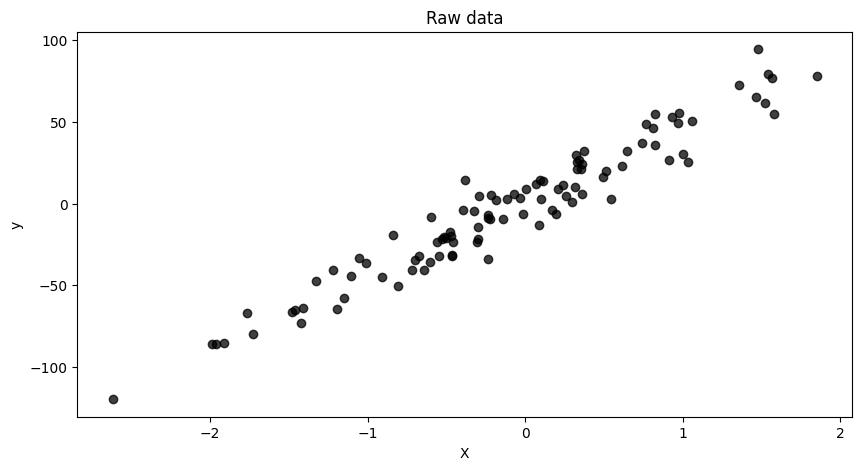
To start, let’s import the libraries we will need and generate some synthetic data using make_regression from sklearn. This will give us a simple dataset where X and y follow a linear relationship, but with some added noise to make it more realistic.

import jax
import jax.numpy as jnp
import jax.random as random
import matplotlib.pyplot as plt
import numpy as np
import numpyro
import numpyro.distributions as dist
from numpyro.infer import MCMC, NUTS, Predictive
from sklearn.datasets import make_regression

X, y = make_regression(n_samples=100, n_features=1, noise=12.0, random_state=42)
X = X.flatten()

Here is a scatter plot of the data:

Now, we define our Bayesian linear model in NumPyro.

def model(X: np.ndarray, y: np.ndarray | None = None):
    """Bayesian linear regression model.

    Args:
        X: Feature vector of shape (N,)
        y: Target vector of shape (N,). Defaults to None (used for predictions).
    """
    slope = numpyro.sample("slope", dist.Normal(0, 10))
    intercept = numpyro.sample("intercept", dist.Normal(0, 10))
    sigma = numpyro.sample("sigma", dist.HalfCauchy(5))

    mean = slope * X + intercept

    # Use plates for efficient vectorization
    with numpyro.plate("data", X.shape[0]):  
        numpyro.sample("obs", dist.Normal(mean, sigma), obs=y)

In our Bayesian linear regression model, we have three key parameters:

• slope: determines how much y changes per unit increase in X.
• intercept: value of y when X = 0.
• sigma: standard deviation of the Gaussian noise in our observations (used in the definition of the likelihood).

Each of these parameters has a prior, our initial belief about what values they should take. If you don’t have a strong initial belief, just set a wide prior (e.g., a normal distribution with a large standard deviation), or hyperoptimize the prior width just like you would do with regularization terms!

Here, I’ve assumed that the slope and intercept follow a normal distribution centered around zero, with a relatively broad standard deviation to allow flexibility. Similarly, I’ve set sigma’s prior to follow a half-Cauchy distribution, which is a common choice for scale parameters in Bayesian models (sigma needs to be strictly positive).

The likelihood of the data is then modeled using a normal distribution centered around the predicted values from our linear equation mean = slope * X + intercept. Each observed data point (y) is assumed to follow a normal distribution centered around this mean, with standard deviation sigma (numpyro.sample("obs", dist.Normal(mean, sigma), obs=y)).

Now comes the exciting part: sampling from the posterior. Instead of estimating a single best-fit line like classical linear regression, we use Markov Chain Monte Carlo (MCMC) methods to sample a range of plausible parameter values from the posterior distribution. The No U-Turn Sampler (NUTS), is often a great choice for this.

# Run MCMC sampling using No U-Turn Sampler (NUTS)
rng_key = random.PRNGKey(0)
nuts_kernel = NUTS(model)
mcmc = MCMC(nuts_kernel, num_warmup=1000, num_samples=2000)
mcmc.run(rng_key, X, y)

# Get posterior samples as dict[str, jax.Array]
samples = mcmc.get_samples()

In the code above:

• num_warmup: the number of initial samples used for tuning the sampler (these are discarded to avoid bias).
• num_samples: the number of valid samples we keep from the posterior.

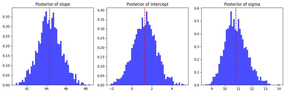
Once we run the MCMC sampler, we extract the posterior samples, which give us a distribution for each parameter. It should look something like:

# print(samples)
{'intercept': Array([ 1.4101534 ,  2.8337934 ,  1.864582  , ..., -0.18940793,
        -0.01620676,  2.2749405 ], dtype=float32),
 'sigma': Array([10.80212  , 11.671823 , 10.161828 , ..., 11.444607 , 11.232727 ,
        10.7905445], dtype=float32),
 'slope': Array([44.500202, 43.78757 , 46.255432, ..., 43.571068, 43.50194 ,
        44.47404 ], dtype=float32)}

Instead of getting just a single best estimate for slope, intercept, and sigma, we now have access to their probability distributions! This is a major advantage of Bayesian inference. Instead of saying: “The slope is 44.5.”, we can say: “The slope is most likely around 44.5, but based on the data, it could reasonably be anywhere between 41.5 and 47.5 with 95% probability.”

This is incredibly useful in practice. In many applications, we care about more than just a point estimate, we want to know how confident we are in our predictions. For example, consider real estate pricing:

• If you’re building a model to predict house prices based on housing surface, your slope would represent price per square meter (\([\$/m^2]\)).
• Instead of just giving a single price estimate, you can provide a range, helping buyers and sellers make more informed decisions.
• A wider range would indicate higher uncertainty, possibly due to limited data or high variability in the market.

This ability to quantify uncertainty is what sets Bayesian methods apart from classical approaches! We can also plot the parameters posterior to see the range of plausible values. This can help us visually understand the model’s uncertainty.

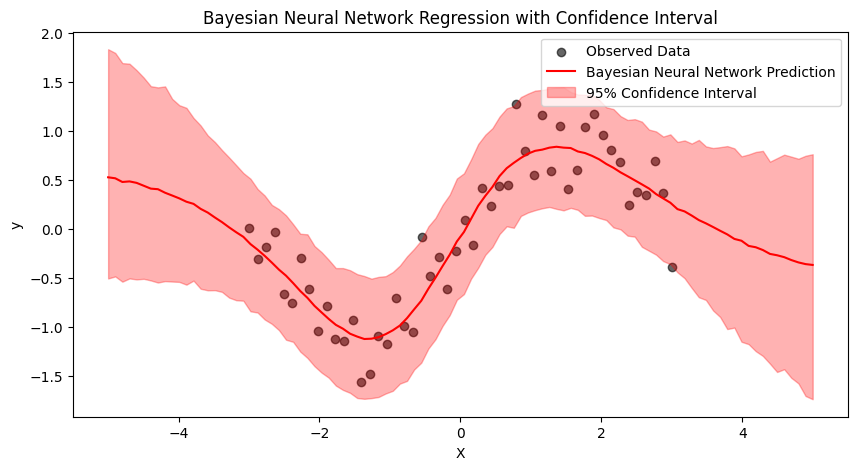
Instead of drawing just one regression line (like in classical machine learning), we can generate multiple likely regression lines based on our posterior samples. A common approach is to plot the mean or median prediction as a solid line, just like you would in a traditional model,but then shade a 95% confidence interval around it. This visually captures the range of possible outcomes and directly shows how much uncertainty there is in our predictions.

Now that we’ve seen Bayesian Linear Regression in action, let’s take things a step further. What if our data isn’t well described by a simple linear relationship? That’s where non-linear model like Bayesian Neural Networks (BNNs) come in! The general idea is similar to what we saw with linear regression, except now the model is a neural network! Here’s a simple shallow network for illustration:

Where \(\mathbf{w}_1\) and \(\mathbf{w}_2\) are are the weights for each layer, and \(\mathbf{b}_1\) and \(b_2\) are the biases.

You can go check the complete Bayesian Neural Network notebook, but here I’ll show you quickly how we can define this model in NumPyro/JAX:

def model(X: jax.Array | np.ndarray, y: jax.Array | np.ndarray | None = None):
    num_hidden = 5

    # Priors for weights and biases of layer 1
    w1 = numpyro.sample("w1", dist.Normal(0, 1).expand([1, num_hidden]))
    b1 = numpyro.sample("b1", dist.Normal(0, 1).expand([num_hidden]))

    # Priors for weights and biases of layer 2
    w2 = numpyro.sample("w2", dist.Normal(0, 1).expand([num_hidden, 1]))
    b2 = numpyro.sample("b2", dist.Normal(0, 1))

    # Neural network forward pass
    hidden = jnp.tanh(jnp.dot(X, w1) + b1)  # Activation function
    mean = jnp.dot(hidden, w2) + b2         # Final output
    mean = mean.flatten()                   # (N, 1) to (N,)

    sigma = numpyro.sample("sigma", dist.HalfCauchy(1))  # Likelihood noise

    with numpyro.plate("data", X.shape[0]):
        numpyro.sample("obs", dist.Normal(mean, sigma), obs=y)

This model defines a simple feedforward neural network. The parameters of the model, weights and biases, are all treated as random variables with prior distributions. By using MCMC (as we did with Bayesian linear regression), we can sample from the posterior distribution of these parameters.

The rest of the code is basically the same as for the linear regression case. I’ve generated some non-linear data for the sake of this example (check the notebook to see the whole code). Here is the plot with the prediction and the 95% confidence interval. Note that we can see that the model is less sure outside the range of seen data!

6. Conclusion

We started this journey by demystifying Bayesian Machine Learning, breaking down its foundations, and showing that it’s not as different from classical ML as it might seem. We’ve seen that it naturally extends classical ML, offering a powerful way to quantify uncertainty and make better-informed predictions.

Here are some key takeaways:

• Bayesian ML can help you make better decisions. Classical ML gives us a single “best guess,” but Bayesian ML tells us how confident we should be in that guess.

• Regularization in classical ML is just a prior in disguise. If you’ve ever used L2 regularization (Ridge regression) or L1 regularization (Lasso), you’ve already been working with priors, even if you didn’t call them that!

• Instead of picking just one model, Bayesian ML averages across all plausible models. This is why Bayesian predictions are often more robust and informative, especially when dealing with small datasets or noisy data.

• Implementing Bayesian ML is easier than you think. With libraries like NumPyro and JAX, you can apply Bayesian techniques to real-world problems without needing a PhD in statistics.

Of course, Bayesian ML is a vast field, and we’ve only scratched the surface. There’s so much more to explore: Variational Inference (VI), Markov Chain Monte Carlo (MCMC), and even Conformal Prediction for classical ML. If this post sparked your curiosity, I encourage you to dig deeper and experiment with these techniques.

Now, let’s be real: Bayesian ML isn’t always the answer. It’s often computationally expensive, and since it’s not as mainstream as classical ML, there are fewer ready-made examples and tutorials available. In many cases, classical ML is the more practical choice, and there are still ways to estimate confidence intervals without going fully Bayesian.

At the end of the day, there’s no “one-size-fits-all” approach in ML. The best method depends on your specific problem, your data, and your constraints. The important thing is that now, hopefully thanks to this blog post, you have a deeper understanding of Bayesian ML, and you can make a more informed decision on when (or when not) to use it. So go ahead, embrace the uncertainty and Bayesian ML!

Enjoy your ML journey! 🚀